
Mob Eraser Removing Villagers from Images in Minecraft
Final Report
Video
Project Summary
The goal of this project is to create a machine learning model to remove villagers from image screenshots taken in minecraft. We want to be able to input an image containing villagers into the model, and have it output an image with no villagers and the background reconstructed as if they were never there.

Machine learning is very useful in this task because it would be very difficult to hard code a program for the infinite amount of villager positions and terrain. Additionally, after removing the villagers from the image, the program must generate a reconstruction of what the background behind the removed villager would look like. A task such as this is infeasible without the utilization of machine learning, since the program must learn how minecraft worlds are laid out and infer the details of the removed section from surrounding attributes and details in the input image. This model could be used to help create screenshots of landscapes in minecraft without having to manually remove villagers or mobs beforehand. It could also be extended to real life scenarios to remove people from landscape shots or remove tourists from personal pictures.
Approaches
Gathering Images
The first step to accomplish was to gather a large dataset of paired images to train on. This was done by writing a malmo program which set the screen size to 256 x 256 pixels and teleported the player to a random location in a normally generated minecraft world. The program then checked if the location was good, such as if the player was not in water, in a wall, or on the side of a cliff. If so, it cleared the current mobs on screen and saved the current image of the screen. Then a random amount of villagers was summoned in random locations and another image of the screen was saved. We then manually scanned through the images afterward and removed poor samples, such as when the world had failed to load. We gathered over 3,000 pairs of images to train on using this method.
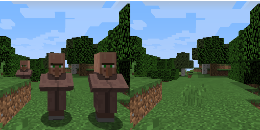
Fig.1 An example of an image pair, one of many used to train and test the models.
Convolutional Autoencoder (CAE)
For our initial model, we created a convolutional autoencoder as a baseline to perform our task. In our model, the encoder took an (256,256,3) tensor as input and was made up of several Conv2D layers with increasing filter size and stride 2 and kernel (2,2), to help with checkerboarding in the reconstruction. The output of the convolutions was then flattened and went through two dense layers to arrive at our compressed latent space representation, which we chose to set at a dimension of 256. The models decoder structure took this latent space vector and passed it through a couple dense layers, and then through some Conv2DTranspose layers that mirrored the encoder’s Conv2D layers and upscaled the compressed representation, resulting in a reconstructed image of the same size, (256,256,3). Our model was compiled with the Adam optimizer with a learning rate of 0.001 and the mean squared error loss function:
The model was then trained with 75% of our collected data for 1000 epochs, where validation was performed using the remaining 25% of the data. As the model trained, we recorded the accuracy and mean squared error for each epoch.
This convolutional autoencoder served as a good baseline model. For the same amount of data that was given to all the models to train and test them, the CAE trained much faster and used less memory. However, the CAE was more prone to overfit the training data, and its images both had a higher error quantitatively, and qualitatively there was a noticeable difference in image clarity, resolution, and sharpness between the CAE and GAN.
Generative Adversarial Network (GAN)
Our second model we developed was a conditional generative adversarial network based on the Pix2Pix architecture. The Pix2Pix architecture is specifically designed for image to image translation, so this type of model should be great to apply to our problem of removing Minecraft mobs. The GAN consists of two main components, the generator, tasked with creating increasingly real-looking images as the model trains, and the discriminator, which attempts to differentiate between real images and images created by the generator.
The generator follows a similar structure to a modified U-Net, where each downsampling block is composed of three layers: a convolutional layer, a batch normalization layer, and a leaky ReLU layer. The upsampling blocks have four layers: a transposed convolutional layer, a batch normalization layer, an optional dropout layer (typically applied to the first couple layers in the decoder), and a ReLU layer. The downsampling blocks compose the generator’s encoder, while the generator’s decoder is made up of the upsampling blocks. Skip connections are implemented between layers in the encoder and decoder as in any typical U-Net.
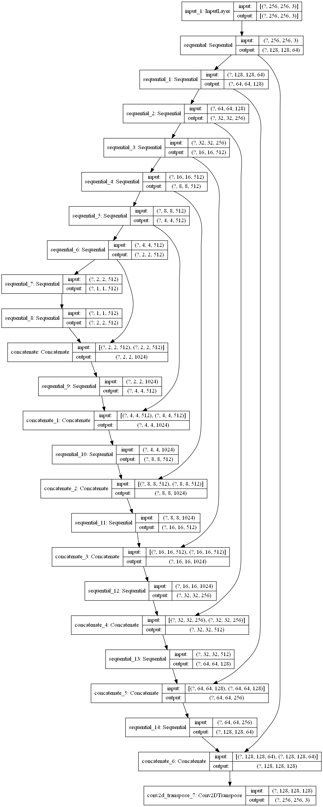
Fig.2 Architecture of the U-Net Generator in our GAN.
The generator loss function is a combination of the sigmoid cross-entropy between the output image and an array of ones, along with L1 regularization. The sigmoid binary cross-entropy is given by the formula:
And L1 loss (MAE) is given by the equation:
The actual formula for the full generator loss is: total_gen_loss = gan_loss + LAMBDA * l1_loss, where LAMBDA is typically set to 100.
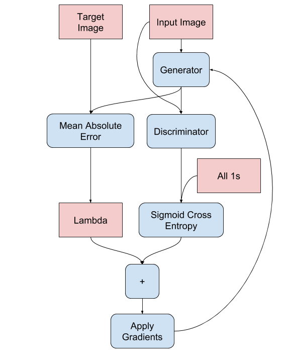
Fig.3 Computational graph of how the Generator loss is calculated.
The discriminator is a PatchGAN, which specializes in penalizing image structure in relation to local image patches. As it is run convolutionally across the image, it tries to determine whether each n x n patch is real or fake, and averages the result to get the final output. Each discriminator block is made up of a convolutional layer, a batch normalization layer, and a leaky ReLU layer, just like the downsampling blocks from the generator.
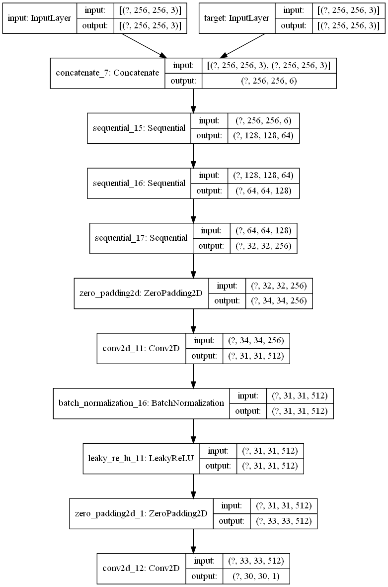
Fig.4 Architecture of the PatchGAN Discriminator in our GAN.
The discriminator loss function is the sum of the sigmoid cross-entropy between the real images and an array of ones and the sigmoid cross-entropy between the fake images and an array of zeros.
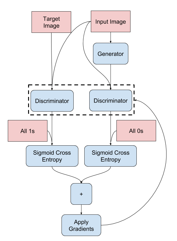
Fig.5 Computational graph of how the Discriminator loss is calculated.
While a GAN trains significantly slower, uses much more memory, and requires a bit more data compared to the CAE due to its increased complexity, it is able to produce much clearer images by retaining the areas of the image which do not change unlike the CAE.
Self-Attention Generative Adversarial Network (SAGAN)
The third and most sucessful model we created was a SAGAN. A SAGAN is a GAN augmented with attention layers and spectral normalization in its convolutional and transposed convolutional layers. Typical convolutional networks are constrained by filter size in their ability to represent image data, but the attention layers enable the generator and discriminator to model relations between spatial regions and capture global dependencies. Often this results in better detail handling and GAN performance.
Each attention layer starts by taking an input tensor of convolution feature maps and creating three copies using a 1x1 convolution corresponding to the key, value, and query. The key is transposed and mutiplied by the query, and the result is fed to a softmax to produce the attention map. This mapping is then multiplied by the value and passed through a final 1x1 convolution to result in an output tensor that represents the new attention feature maps.
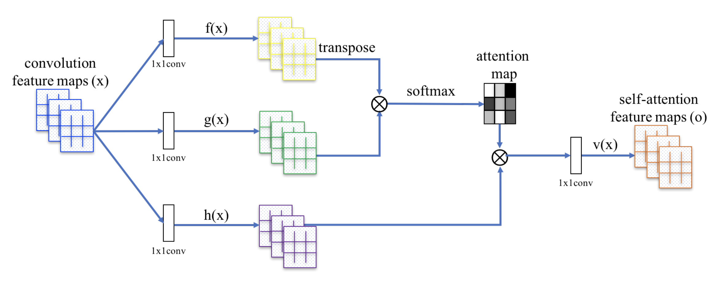
Fig.6 Architecture of an attention layer.
Spectral Normalization is a weight normalization technique that attempts to mitigate standard problems GANs often face, most typically the expoding gradient and mode collapse problems. This method stabilizes the GAN training epochs by controlling the Lipschitz constant of the discriminator. Spectral normalization normalizes the weight for each layer with the spectral norm, forcing the Lipschitz constant for each layer and the whole network to be equal to one. In doing so, the gradient is prevented from changing drastically and pulling the GAN away from reasonable values.
We implemented our SAGAN with both spectral normalization on the colvolutional and transposed convolutional layers and with attention layers in the generator and discriminator. Compared with our previous GAN, the SAGAN performed very slightly better, likely due to its inherant ability to map relations between larger spatial regions than the limited kernel size of the convolutional layers, so it was able to understand more of the “rules” behind how the images are constructed and better reconstruct the missing data behing the removed mob. Qualitiatively, if you look closely at images generated by the GAN and SAGAN, you will notice that the GAN his slightly more pixelation and a bit worse color accuracy when it comes to the area where the mob once resided.
Evaluation
Quantitative
As mentioned earlier, our CAE model was tested on 25% of our collected data that we set aside to evaluate its performance. Our two main quantitative metrics we used to evaluate the convolutional autoencoder’s performance were binary accuracy between image pixels and mean squared error between the expected and reconstructed images. One point of evaluation was checking the recorded accuracy and mean squared error values we recorded during our training epochs to ensure the model was training properly, showing clear progress, and was not overfitting or underfitting the data.
Fig.7 Binary pixel accuracy and MSE of the CAE over its 1000 training epochs.
From the above diagrams, we can see that the accuracy and MSE kept improving, but significantly tapered off after around 450 epochs, meaning the returns for each epoch were minimal, so we began to slightly overfit the training data. If we continued to train the CAE for more epochs, we would overfit the training data more and more, which would cause serious problems when we attempted to run the model on non-training data, like our testing dataset.
As for the GAN models, we monitored the four loss criteria we outlined in the preceding discussion. The loss criteria we monitored for the generator were gen_total_loss, or the total GAN generator loss, gen_gan_loss, or the cross-entropy loss from the generated image and ones, and gen_l1_loss, or the l1 regularized loss between the gan image and target. The loss criteria for the discriminator was disc_loss, or the total GAN discriminator loss. We expected that the values of gen_l1_loss and gen_total_loss would keep decreasing, similar to the accuracy or MSE from the CAE.
Fig.8 Loss metric diagrams taken from 100 epochs of GAN training.
As we trained the model, we looked for specific details in the above graphs to check whether the GANs were behaving properly. First, we checked to make sure there was no drastic difference between the gen_gan_loss and disc_loss, since if either loss became very small, it would indicate that one model was dominating the other and the GAN is not trainign properly. We also checked that these losses were around the value 0.69, since this value indicates a preplexity of 2, meaning that specific model had a 50% chance of fooling the other model. Any value lower would indicate that the model was doing better than random, and any value higher indicated the opposite. Our gen_gan_loss ended up around 0.70, which means it was pretty close to fooling the discriminator 50% of the time, which is right where we wanted it. The disc_loss settled around 1.4, meaning it was doing slightly worse than random on the combined set of real and fake images, which isn’t excatly ideal, but is not too unordinary that it caused concern. Gen_l1_loss followed the expected trajectory of decreasing as time went on, and since gen_total_loss is the sum of gen_gan_loss and gen_l1_loss, it also decreased as expected. Ultimately, our GAN model trained well and mostly met with our expectation regarding its numerical performance.
Qualitative
Additionally, we also visually inspected the recreated images and compared them to the expected result to see how the model was improving and how effective the output was to a human observer, as the whole premise of the project is to remove mobs from screenshots to help people create better and less cluttered images. The CAE images serve as a great functional baseline for our image reconstruction, as they sucessfully remove the mob from the image and fill in the missing portion in a similar manner to which the surrounding environment looks like.
Fig.9 Sample input, expected, and reconstructed output images from the CAE testing.
However, our GAN images were much clearer and more representative of what one would expect from removing a Minecraft mob. While the CAE struggled with detail loss, noise, and compression when it tried to output sharp images, the GAN was able to capture the original image details flawlessly, minus the exact silhouette where the mobs resided, which had some slightly noticeable pixelation.
Fig.10 Sample input, expected, and reconstructed output images from the GAN testing.
Directly comparing the images produced by the CAE (top) and the even better SAGAN (bottom) easily illustrates the disparity in effictively reproducing the images. The CAE images successfully removed the mobs and generated new background where they once were, but the entire reconstructed image comes out pixelated and noisy. In contrast, the SAGAN images are sharp and clear, with very little errors where the mobs once were. The difference in feature representation is due to the complexity and abilties of the two different models. The CAE is great for dimensionality reduction, image denoising, and anomaly detection on small images, but the GAN, especially the Pix2Pix architecture, was specifically designed to translated between images, and was suited perfectly to our task, and it shows in the results.
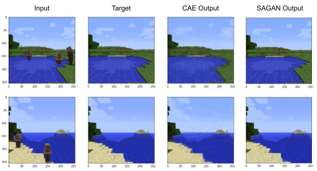
Fig.11 Input, target, and output for the CAE (third column) and SAGAN (fourth column).
Resources
- https://microsoft.github.io/malmo/0.30.0/Schemas/MissionHandlers.html#type_GridDefinition
- http://microsoft.github.io/malmo/0.30.0/Documentation/
- https://minecraft.gamepedia.com/Game_rule
- https://www.youtube.com/watch?v=FEB8nUzwCSA&feature=youtu.be
- https://microsoft.github.io/malmo/0.17.0/Documentation/structmalmo_1_1_world_state.html#a2d2c915c1aa01eb3856924b35ae02591
- https://www.tensorflow.org/tutorials/generative/autoencoder
- https://www.tensorflow.org/tutorials/generative/dcgan
- https://www.tensorflow.org/tutorials/generative/pix2pix
- https://lilianweng.github.io/lil-log/2018/06/24/attention-attention.html#self-attention-gan
- https://jonathan-hui.medium.com/gan-spectral-normalization-893b6a4e8f53
- https://arxiv.org/abs/1802.05957
- https://arxiv.org/abs/1805.08318
- Malmo depth_map_runner.py sample program
- Python version 3.7.2
- Python packages: TensorFlow 2.1.0, Numpy 1.18.1, Pillow 5.4.1, Matplotlib 3.2.1, Notebook 6.0.3